
My Research
Computational Fluid Dynamics and Numerical Methods Research
Since January 2024, I have been applying my experience in MATLAB and fluid dynamics to computational mathematics research under Swarthmore professor Dr. Joseph Nakao. I am currently developing a novel high-accuracy, implicit, low-rank solver for the Vlasov-Dougherty-Fokker-Planck system in cylindrical coordinates, which has applications in plasma simulations. More general Vlasov-Fokker-Planck-type equations can be extended to model nuclear fusion, a research area I am especially drawn to because of its renewable energy applications.
Plasma dynamics and fusion interaction models require systems of nonlinear PDEs. However, analytically solving nonlinear PDEs is often impossible, and experiments are resource-intensive, necessitating high-accuracy numerical solutions. Ideally, these solutions must capture sharp gradients, conserve physical structures (e.g. mass, momentum, energy), and maintain the positivity of the solution. Numerical solutions also suffer from the curse of dimensionality: increasing the numerical solution’s dimensions causes exponential growth in computational cost. Plasma systems of interest are described in up to six-dimensional phase space–plus time–via probability density function $ f(x, v, t) $, which describes the likelihood particles exist at position $ \mathbf{x} \in \mathbb{R}^3 $ with velocity $ \mathbf{v} \in \mathbb{R}^3 $ at time $ t > 0 $.
Vlasov-Fokker-Planck Plasma System
The model
We are interested in solving the Vlasov-Fokker-Planck (VFP) equation to model single-ion plasmas in 1 spatial and 2 velocity dimensions in cylindrical coordinates:
\[\begin{cases} \partial_t f + \mathbf{v} \cdot \nabla_x f + \mathbf{E} \cdot \nabla_v f = C_{\alpha \alpha}(f, f) + C_{\alpha e}(f, f)\\ C(f, f) = \nabla_v \cdot \Big( (\mathbf{v} - \mathbf{u})f + \left(\mathbf{D} \nabla f \right)\Big), \quad (\mathbf{x}, \mathbf{v}) \in \Omega = \Omega_{x} \times \Omega{v}, \quad t > 0 \end{cases}\]where the solution $f(x, v_\perp, v_\parallel, t)$ is the ion probability density function in space and velocity
$\mathbf{E}$ = electric field
$C_{\alpha \alpha}(f, f)$ = ion-ion advection-diffusion Fokker-Planck collision operator.
$C{\alpha e}(f, f)$ = ion-electron advection-diffusion Fokker-Planck collision operator.
![]()
This equation is also coupled with the fluid electron pressure equation. All systems depend on the system’s zeroth, first, and second moments: mass/number density $n$, momentum $nu_{\parallel}$, and ion temperature $T_\alpha$, as well as the electron temperature $T_e$.
Numerical discretization
We discretize the Vlasov-Fokker-Planck equation over a spatial and velocity mesh:
Spatial mesh: Cells $[x_{i-\frac{1}{2}}, x_{i+\frac{1}{2}}] $
Velocity mesh: Cells $ [v_{\perp, j-\frac{1}{2}}, v_{\perp, j+\frac{1}{2}}] \times [v_{\parallel, l-\frac{1}{2}}, v_{\parallel, l+\frac{1}{2}}]$
where the numerical fluxes $\hat{f}^k_{i \pm \frac{1}{2}}$ are computed using a standard first-order upwinding scheme to determine the system’s velocity in the $x$ dimension.
Storage complexity and the curse of dimensionality
Naively, the full-rank solution with spatial size $N_x$ and velocity size $N_v$, the storage complexity is $\mathcal{O}(N_x N_v^2)$, or $\mathcal{O}(N^3)$ if $N_x = N_v = N$.
To avoid the curse of dimensionality, i.e. prohibitively large storage complexity due our equation’s high-dimensionality, we use a low-rank framework to numerically solve the time-dependent partial differential equation. In plasma physics applications, the solution is typically low-rank in velocity and we can decompose the solution into its bases in $V_{\perp}$ and $V_{\parallel}$ and singular values:
\[\mathbf{f}^{k}_i = \mathbf{V}_\perp^{k}\mathbf{S}^{k}(\mathbf{V}_\parallel^k)^T\]Assuming low-rank structure ($r \ll N_v$) $\to$ Storage complexity reduction: $\mathcal{O}(N_x(r^2+2N_vr))$
Newton method and fluid solver
Because the stiff collision and Lorentz force operators require us to use implicit Runge-Kutta methods, we need to compute the moments $(n^{k+1}), ((nu_{\parallel})^{k+1}), (T_\alpha^{k+1}), (T_e^{k+1})$ at future time-steps. Thus, we incorporate a fluid solver that explicitly solves the VFP and fluid electron pressure equation system, analytically integrated to model the zeroth, first, and second moments. We use temporally second-order diagonally implicit Runge Kutta (DIRK2) method to compute these moments at future timesteps.
| Quantity | Δt | L1 (global) | Mass | Momentum | Ion Temp | Electron Temp |
|---|---|---|---|---|---|---|
| L1 error | 0.20 | 0.148 | 0.956 | 0.128 | 0.983 | 0.563 |
| 0.10 | 0.037 | 0.240 | 0.032 | 0.245 | 0.139 | |
| 0.05 | 0.009 | 0.060 | 0.008 | 0.061 | 0.034 | |
| 0.025 | 0.002 | 0.015 | 0.002 | 0.015 | 0.009 | |
| Order | 0.20 → 0.10 | 2.007 | 1.992 | 2.014 | 2.003 | 2.023 |
| 0.10 → 0.05 | 2.003 | 1.996 | 2.006 | 2.002 | 2.011 | |
| 0.05 → 0.025 | 2.001 | 1.998 | 2.003 | 2.001 | 2.005 |
Timestepping procedure
At each timestep $t^k$:
- Compute moments at next timestep $(n^{k+1}), ((nu_{\parallel})^{k+1}), (T_\alpha^{k+1}), (T_e^{k+1})$ using Newton method
At each spatial node $(x_i)$:
- Compute numerical fluxes $(\hat{f}^k_{i \pm \frac{1}{2}})$
Compute electric field:
\(E_{\parallel}^{k+1} = \dfrac{1}{q_{e}n_{e}^{k+1}} \dfrac{(n_{e}T_{e})_{i+1}^{k+1} - (n_eT_{e})_{i-1}^{k+1}}{2 \Delta x}\)- Compute collision operators $(C_{\alpha\alpha}^{k+1}, C_{\alpha e}^{k+1})$
Solve for $(f_i^{k+1})$ using low-rank projection [1]:
Basis update
$K^k = V_\perp^k S^k (V_{\parallel}^k)^T V_{\parallel,\star}^{k+1}$$L^k = V_\parallel^k (S^k)^T (V_\perp^k)^T V_{\perp,\star}^{k+1}$
Galerkin projection
$S^k = (V_{\perp,\star}^{k+1})^T V_\perp^k S^k (V_\parallel^k)^T V_{\parallel,\star}^{k+1}$- Solve for $(K^{k+1}, L^{k+1}, S^{k+1} \mapsto V_\perp^{k+1}, V_\parallel^{k+1}, S^{k+1})$
- Apply conservative truncation procedure [2]
Numerical Tests
We test our solver on a standing shock problem, where the solution is initialized as a Maxwellian moments (mass, momentum, energy) at each spatial node are initialized as hyperbolic tanget equations in space
Numerical solution at time t=200:

Mass, momentum, and energy conservation (up to truncation tolerance):

Mass, momentum, and energy of the system across space, evolved over time.
![]()
![]()
![]()
Most recently presented at SIAM NNP 2025 Conference poster session:
References
[1] Nakao, J., Qiu, J.M. and Einkemmer, L., 2025. Reduced Augmentation Implicit Low-rank (RAIL) integrators for advection-diffusion and Fokker–Planck models. SIAM Journal on Scientific Computing, 47(2), pp.A1145-A1169.\
[2] Guo, W. and Qiu, J.M., 2024. A Local Macroscopic Conservative (LoMaC) low rank tensor method for the Vlasov dynamics. Journal of Scientific Computing, 101(3), p.61.
The Dougherty-Fokker-Planck Equation
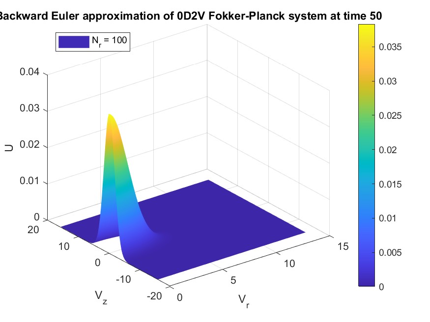
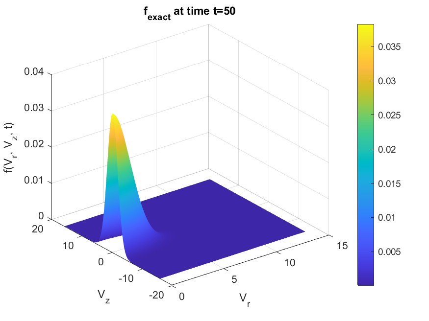
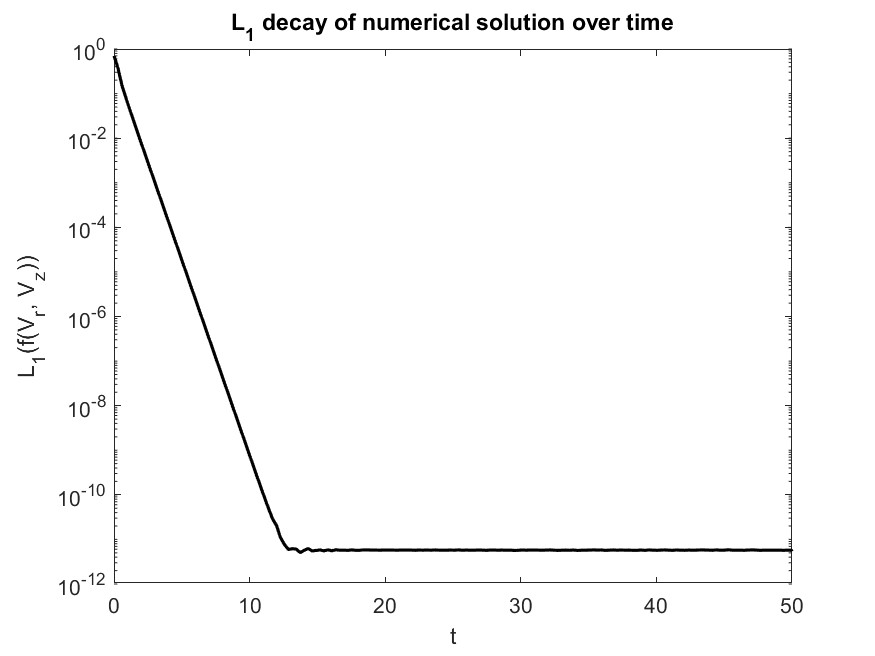
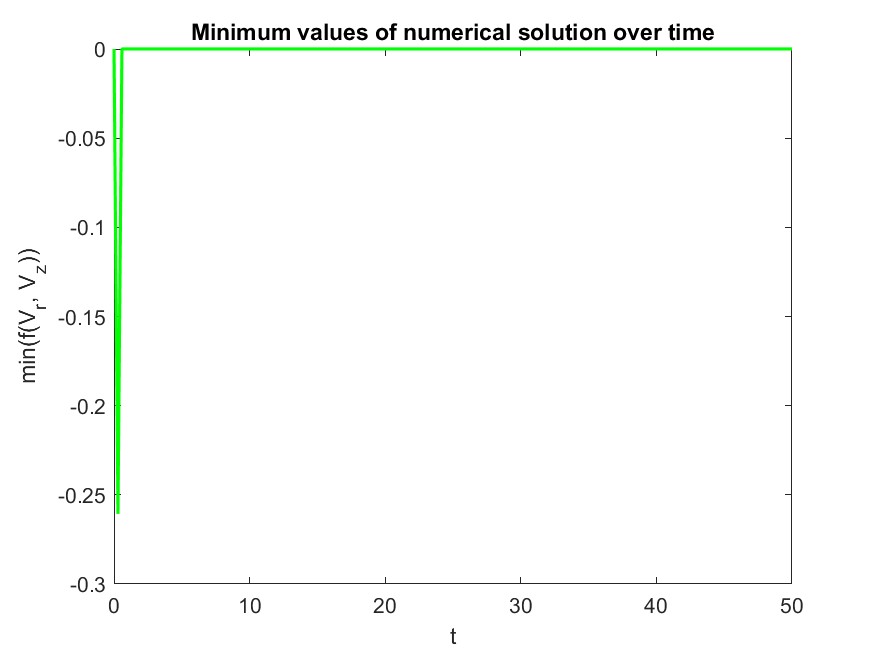
During Fall 2024, as a first step, I worked to develop a low-rank, implicit, structure-preserving solver for the spatially homogeneous 0D2V (zero spatial, two velocity dimensions) Dougherty-Fokker-Planck equation:
\[\begin{cases} f_t = \nabla_v \cdot \Big( (\mathbf{v} - \mathbf{u})f + \left(\mathbf{D} \nabla f \right)\Big), \quad \mathbf{v} \in \Omega, t > 0 \\ f(\mathbf{v}; t=0) = f_0(\mathbf{v}), \quad \mathbf{v} \in \Omega \end{cases}\]in cylindrical coordinates with assumed azimuthal symmetry. $ \mathbf{D} $ is the anisotropic diffusion tensor and $ \mathbf{u} $ is the bulk velocity. While the above equation is spatially homogeneous, future goals involve solving the spatially inhomogeneous 1D2V Vlasov-Dougherty-Fokker-Planck equation.
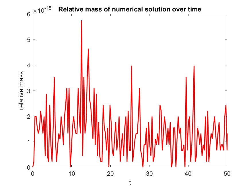
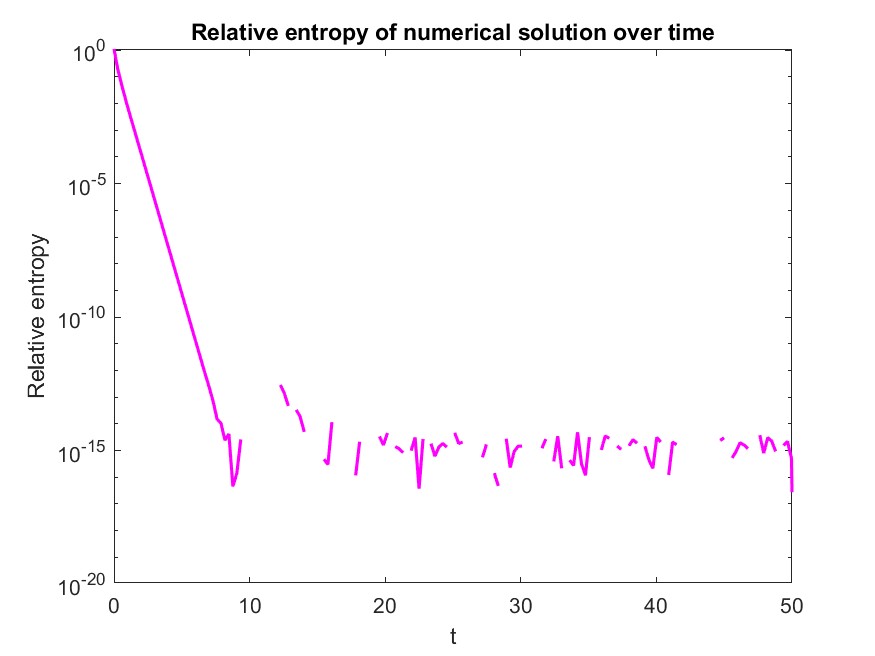
The preliminary results below demonstrate preservation of mass, high-order drive to the correct equilibrium solution (L1 decay), and positivity preservation for the probability distribution. Note that mass and positive are preserved to the system’s truncation tolerance $ 10 ^{-6} $, and the numerical solution’s L1 decay and relative entropy drivee to the same tolerance, indicating physical relevance.
Electrical engineering research - oscillatory wind-energy harvesting device
During spring 2024, I collaborated with fellow physics and engineering students under Swarthmore Engineering Professor Dr. Emad Masroor, developing a small-scale, oscillatory, wind-powered energy harvester. I brainstormed and improved the device’s design, which ultimately comprised a metal chassis holding a 3D-printed cylinder that oscillates perpendicularly to wind flow on vertical springs due to the vortex shedding patterns induced by the airflow across the cylinder itself. These oscillations move small neodymium magnets through wire coils to generate voltage according to Faraday’s law of induction. I used ViscousFlow to investigate vortex-shedding patterns over various shapes to optimize the cylinder’s shape and dimensions. I also researched electromagnetic induction and used MATLAB to model how changes in magnetic field strength, oscillation frequency, and amplitude affect the device’s output power. I validated these theoretical predictions using an Arduino-controlled model that I designed using 3D-CAD software to analyze the effect of different oscillation frequencies and amplitudes on power output. I varied the oscillation parameters of a neodymium magnet passing through the wire coil and analyzed the output voltage data using MATLAB. I used this data to optimize the device’s natural frequency and amplitude parameters, which informed the energy harvester’s optimal spring constants and lengths. Our team also tested device prototypes in the Swarthmore wind tunnel to determine the optimal wind speeds for the highest electrical power output.
Brainstorming, designing, and developing the oscillating test model improved my skills in embedded system design, CAD software, Arduino, and MATLAB, while analyzing the device’s electromagnetic induction system advanced my experimental and theoretical knowledge of fluid dynamics, aerofoils, and electromagnetism. The project also motivated me to research the computational aspect of fluid dynamics and plasma physics, utilized in nuclear fusion energy generation.